
Example |
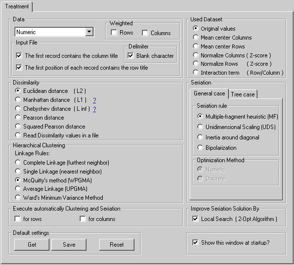
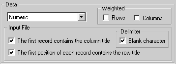
Type | Numeric | The input file contains numerical data. | |
| Binary | The input file contains binary data.(Option not implemented yet) | |||
| Delimiter | In the data file, blanck characters are interpreted as delimiters. | |||
| Input File | The first record contains the column identifiers. | |||
| The first column contains the row identifiers. | ||||
| Weighted | Rows | Rows are weighted. |
||
| Columns | Columns are weighted. Place the weights of each column in the first numerical row, just after the column identifiers. |
|||
1 - Numerical Data
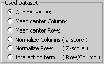 |
Original values |
The graphical representation is based on the raw data of the input file, without any transformation. |
Mean center Columns |
The graphical representation is based on column-centered data: column mean is subtracted from each value, so that mean value of each column is 0. |
|
Mean center Rows |
The graphical representation is based on row-centered data: row mean is subtracted from each value, so that mean value of each row is 0. | |
Normalize Columns (Z-score) |
The graphical representation is based on Z-scores. Columns are standardized to have mean 0 and standard deviation 1. |
|
Normalize Rows (Z-score) |
The graphical representation is based on Z-scores. Rows are standardized to have mean 0 and standard deviation 1. |
|
Row-column interactions |
The graphical representation
is based on data after subtraction of row and column deviation. |
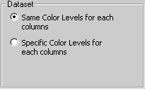 |
Same Color Levels |
The graphical representation is based on the raw data of the input file, without any transformation. |
Specific Color Levels |
The graphical representation is based on column-centered data: column mean is subtracted from each value, so that mean value of each column is 0. |
|
| |
TOP |
1
- Numerical Data |
|
Distances or Index of dissimilarity used for clustering and seriation |
|
Euclidean distance |
 |
http://en.wikipedia.org/wiki/Euclidean_distance | |
Manhattan distance |
|
http://en.wikipedia.org/wiki/Taxicab_geometry | |
Chebyshev distance |
http://en.wikipedia.org/wiki/Chebyshev_distance | ||
Pearson distance |
Clustering, and seriation methods,
are based on Pearson disimilarity s =1-r, where r is
the usual Pearson correlation coefficient. This metric varie between 0
and 2. |
||
Squared Pearson distance |
Clustering, and seriation methods,
are based on Pearson disimilarity |
||
Jaccard's distance |
http://en.wikipedia.org/wiki/Jaccard_coefficient | ||
Dice's dissimilarity indice |
http://en.wikipedia.org/wiki/Dice's_coefficient | ||
Read dissimilarity values from a file |
If you want a special distance,
or dissimilarity, you can compute your own distance or dissimilarity values
with another application and import these values in PermutMatrix from
a file. This file must be a triangular matrix in a standard text file
format (ASCII) as for data file format. |
||
 |
aggregation criteria |
||
|
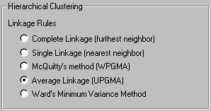
Complete linkage |
The distance between two classes A and B is the maximum of all pairwise distances between items contained in A and B. |
||
|
Single linkage |
The distance between two classes A and B is the minimum
of all pairwise distances between items contained in A and B. |
||
|
McQuitty 's method (WPGMA) |
The distance between two classes A and B is
an weighted mean of all pairwise distances between items
contained in A and B. The distance of a group of two classes A and B to
a class C is the unweighted average of the distances between A and C on
one hand, and B and C on the other. |
||
|
Average linkage (UPGMA) |
The distance between two classes A and B is
the unweighted mean of all pairwise distances between
items contained in A and B. So, the distance of a group of two classes
A and B to a class C is the average of the distances between A and C on
one hand, and B and C on the other hand, the average being weighted by
the size of each class. |
||
|
Ward's minimum variance |
At each aggregation step, the lowest variation of intra-class inertia is searched. |
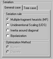 |
Seriation Criteria: |
|
|
|
|
Multiple-fragment heuristic do not guarantee to find an optimal solution but give quickly a "reasonable good" solution. In PermutMatrix the Multiple-fragment heuristic can be improved by the "2-Opt" local search algorithm.
| Check these boxes to execute automatically the specified seriation method
after a hierarchical clustering. If these boxes are checked, Hierarchical clustering and seriation will be performed automatically after any modification of options parameter. |
|
| At any time, you are able to run cluster analysis, followed automatically by seriation, using the keyboard shortcut : F6, for rows reorganisation; Shift + F6 for columns reorganisation; F7 for both. | |
| PermutMatrix |
|